Chapter 13 Bayesian inference
Is it enough to process information down the network? No. Cause can by definition only flow down it. But we might have information which implies something about antecedents, which means we have to reason backwards.
Arrows can be coded with information on specificity and sensitivity, so we can use Bayes’ rule to modify our prior information about the upstream variable(s).
Not implemented, but soon.
It’s the same for specifying the contour:
- straight:
(contour=straight)(the default. I don’t say “linear” as that can mean other things too) - quick-start:
(contour=quick-start) - slow-start:
(contour=slow-start) - S-shaped:
(contour=S-shaped) - U-shaped:
(contour=U-shaped) - threshold:
(contour=threshold)
… and each of these options can be reversed, e.g. “reversed straight” ( = NOT for binary variables).
Consequence variable
.(contour=U-shaped) Some influence variable
.(contour=reversed straight) Another influence variable 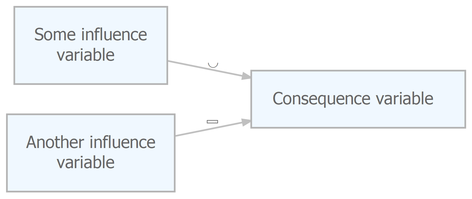
13.1 Specifying the strength of individual influences
Each causal link can have a “strength”, default 100%, otherwise less. e.g.:
Consequence variable
.(contour=reversed straight; strength = .5) Some influence variable
.(contour=reversed straight) Another influence variable 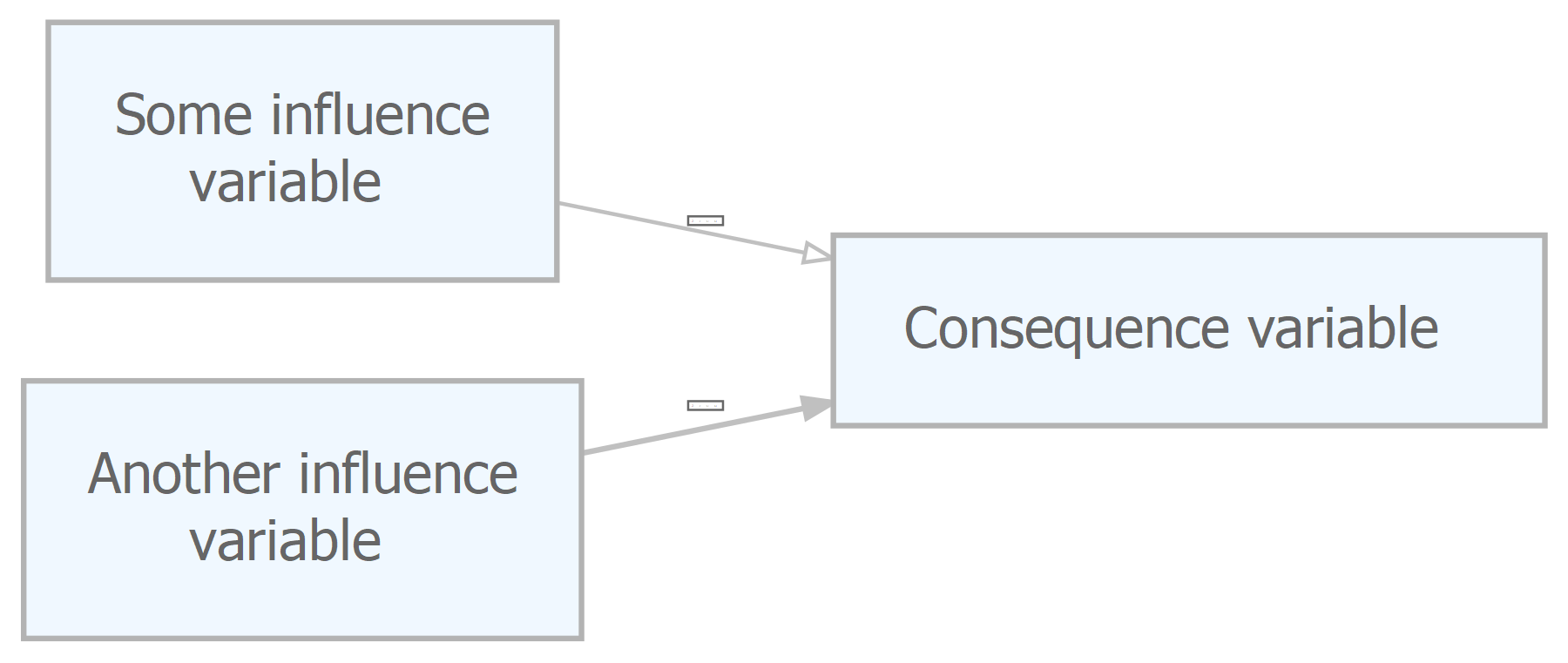
The default is strength=1. Arrows with strength less than 1 are shown correspondingly thinner and with a different arrowhead. (This can be overridden by specifying the width directly, e.g. by adding width=4)
13.2 Specifying the residual
If any of the “strengths” of the incoming links is less than 100%, there is an additional “residual” setting for the consequence variable. Because otherwise, the value of the consequence variable is not fully specified - the shape of the function becomes squashed and doesn’t take up the whole y-axis. So for example, if the maximum incoming strength is 50%, the residual (also between 0 and 100%) can shift the squashed function up to about 50% up and down the y-axis.
Consequence variable; residual=1
.(strength = .5) Some influence variable
.(strength = .5) Another influence variable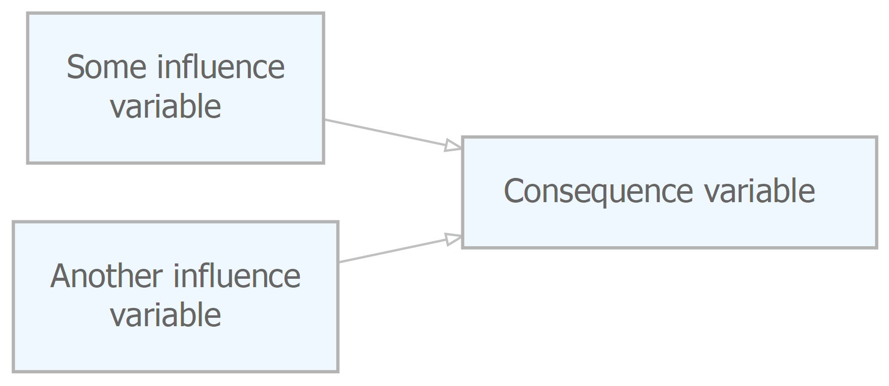
13.3 Combinations: Ways in which the consequence variable can combine its influences
- hard-add (just addition, but cuts off at 100%)
- soft-add (the default: a kind of poor man’s sigmoid, but nicer because it can actually reach 0 and 100% unlike sigmoids)
- multiply (the same as AND in the special case of binary variables)
- smallest (also the same as AND in the special case of binary variables)
- largest (the same as OR in the special case of binary variables)
- average
- similarity (a measure of dispersion, so if all incoming variables are the same, the similarity is 100%)
e.g.
Consequence variable (combination=multiply)
.(contour=reversed straight; strength = .5)Some influence variable
.(contour=reversed straight)Another influence variable 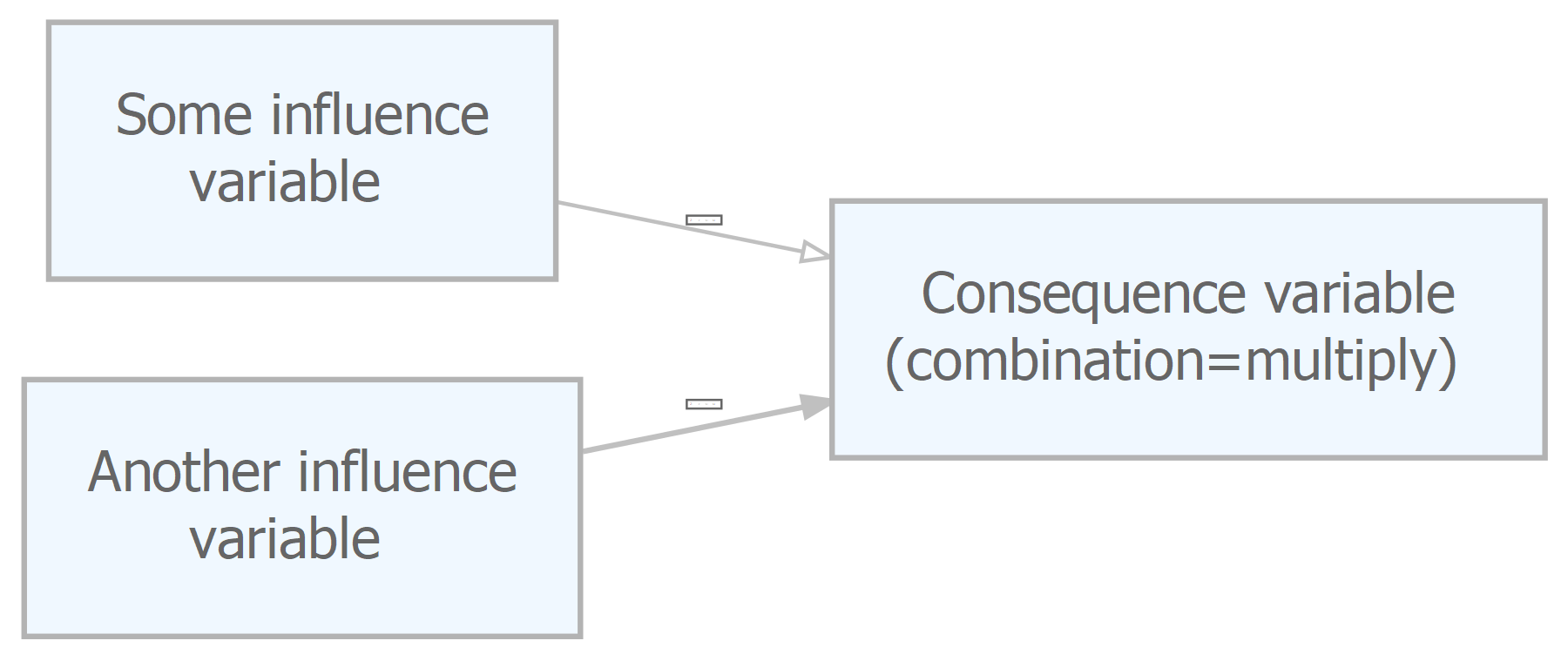
13.4 Flipping
Also, each consequence variable can be “flipped” in relation to the combination of its incoming variables. (We say “flipped” because the word “reversed” is used for the incoming contours). All of these combinations work with any number of incoming variables greater than 1).
13.5 Shortcuts
We so often set variables to ; intervention=1; base=0 that there is a special shortcut for that: just type !tick after the variable name:
My variable !tickType (.9--.3) after a variable name to designate a variable as ; intervention=.9; base=.3.
Type (--.3) to designate a variable as base=.3.
So this:
Variable 1 (1--0)
Variable 2 ( --0)
… means that we intervene to set Variable 1 to 100% rather than 0%, and that variable 2 just has a base level of 0, we don’t intervene on it.