Theorymaker - a language for Theories of change.
Steve Powell

Overview of sections
Village resilience as a defined Variable

This is similar to the previous diagram. Now two orange boxes are used just help to organise the diagram. They are not part of the causal story.
Resilience is now shown as a Variable in its own right, but as something defined in terms of income and flood risk rather than caused by them. Defined Variables are shown with dashed lines.
To assess resilience (in this model) we would just assess flood risk and income and combine the information in some way: it wouldn’t make sense to measure resilience separately, so it is given a dashed border. (For example, we might conceive of resilience as being somehow the “sum” or “average” of the two contributing Variables. However, this diagram is about the underlying ideas, not on the details of measurement or “indicators”.)
Resilience is not shown as being valued in its own right in this case - it has no ♥ or 🙁 symbol - it is merely valuable because the other two Variables are.
Village resilience: all or nothing

This diagram is similar to the previous one. But this time, flood risk and family income are not valued on their own (they have no “♥” or or “🙁” symbol) and they are conceived of as all-or-nothing. If both these things happen (their arrows are joined and have an “AND” symbol) we declare that the village is now “resilient”, again presented as a simple case of yes or no (“◨”). As in the previous example, resilience is not conceived of as a further Variable downstream which is causally influenced by income and flood risk. Instead, it is defined in terms of them. And this time, we do not care about the flood risk or the family income on their own: we only care about this critical level of resilience, perhaps because our funding depends on it.
The management of a project with this Theory of Change might behave quite differently from the previous example:
- Once a village achieved the critical income target, work on that could stop in favour of work on the flood preparation target, and vice versa
- Once one village achieved this critical resilience target, it would no longer be interesting for project management, who might focus on other villages
Village resilience: showing the Difference made by a project

This diagram is similar to the first one, but now each Variable also presents information about projected performance with and without the project. We might see this kind of diagram after the project is over as the summary of an evaluation. Or we might see it before the project has even begun, as a way of expressing targets - what we hope to be able to achieve: the Difference we will make.
The ✔ symbol shows that the intervention happens rather than not happening. The Difference made to family income has even been quantified: $5 rather than 4. This “$4” is what would have happened without the project, which is not necessarily the baseline score, as income might be changing anyway.
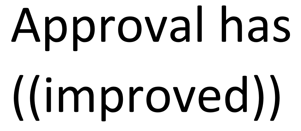
In Theorymaker, we usually express Differences within double brackets, either as a summary such as, say, “improved” or as a formulation with “rather_than” (like we did here for flood risk). The ✔ also shows a Difference - implemented rather than not implemented.
SECTION 3: Main symbols and elements


Variables: things that could be different
Variables: things that could be different. We represent them with words written inside simple shapes, usually rectangles. They are the basic building blocks of Theories. Ideally we also indicate the range of possible Levels the Variables can take (e.g. yes and no, low through to high, etc). We call them Variables - with a capital V.

This kind of network diagram can be very useful but these rectangles are not Variables but things.

Now, these are Variables. They can take different levels or values:
- here, one Variable can be zero or very high, or anywhere in between.
- the other can be only “for” or “against”
In these slides we will not distinguish much between the Variables and Theories as communicative acts, i.e. things we write down and share, and what they represent.
Conventional descriptions of Theories of Change rarely discuss what their basic elements actually consist of.
Simple Theories: showing the causal influences of one or more influence Variables on a consequence Variable
We use arrows to link one or more Variables (the “influence Variables”) to another (the consequence Variable"). Meaning: the influence Variables causally influence the consequence Variable: if you manipulate the influence Variables, this will make a difference to the consequence Variable. The combination of influence and consequence Variables (and the arrows joining them) is called a simple Theory (with a capital T).
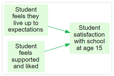
This diagram shows how two Variables influence another Variable …"

“How satisfied is the student? It depends on their feeling of support, of living up to expectations , …”
Simple Theories are nuggets of practical information about the influences on a Variable:
- more or less accurate rules of thumb, help us to understand how the world works
- more or less general or specific
It’s our job to provide the best Theories with the best evidence! In any give situation, many different, overlapping Theories can usually be applied.
Essentially, a simple Theory is nothing more than an equation of the form
V=f(U1,U2...) | C
which expresses some variable V in terms of some other variables U1, U2 … via a function f (given a particular context C). For example,
Student satisfaction with school =
f(How much student feels that they live up to expectations,
How much student feels supported and liked)
The fun starts when we ask about the nature of these variables, what kinds of functions are allowed, etc. Theorymaker points out that even when many of these things are not completely defined, still we can do some reasoning with sets of such equations - see Soft Arithmetic.
How do we express the causal relationship? It isn’t equality
\[V=f(U1,U2...) |C\]
This “=” is neither equality nor logical implication.
Our causal knowledge is captured by:
\[acceleration=f(force) |mass=m\]
… but, surprisingly, not (at least, not in the same way) by:
\[mass=f(force) |acceleration=a\]
… because if we intervene to change the acceleration, we don’t change the mass.
How do we express the causal relationship? It isn’t logical implication.
This logical implication is true (because if the left-hand-side of an implication is true, the whole expression is true.)
\[We\,are\,on\,planet\,Earth\, \Rightarrow \, The\,sky\,is\,green\]
… but it doesn’t capture any causal knowledge:
Joining together simple Theories into composite Theories


… we can join them together into a “composite Theory”.
A composite Theory is two or more simple Theories “snapped together” (providing there are no loops): ℹ This does not mean we can’t introduce “feedback loops”. See later. The resulting network is a DAG - a Directed Acyclic Graph, see (Pearl 2000)

A Theory is either a simple Theory or a composite Theory.
So as a composite Theory is just a set of simple Theories, from a formal point of view, a composite Theory is just a set of equations (see the “Fundamentals” tab in the previous slide)
So, given a set of separate simple Theories,
\[V=f(U1,U2...) |C\] \[W=f(X1,X2...) |D\] …
… we get a single, composite Theory, which is true in the intersection of the contexts.
\[V=f(U1,U2...) |C \cap D\] \[W=f(X1,X2...) |C \cap D\]
“…|C” means “given a particular context C”.
(“Ministeps”: (Birckmayer and Weiss 2000))
Talking about Theories using Words in Capitals: Variable, Theory …
In the previous slides, we saw these words …
- Variable
- Simple Theory
- Composite Theory
- Theory
… introduced for the first time in bold, together with their meanings.
We will use these words (in capitals)ℹ More technically, these Words in Capitals are part of the Theorymaker meta-language to speak about the diagrams we will see in these Theorymaker slides.
We also saw how the Variables at the beginning of a simple Theory are called the “influence Variables” and the other Variable is called the “consequence Variable”. These are useful extra words for talking about the parts of a simple Theory.
Also, we call Variables “at the end” of a Theory, which have no consequence Variables “no-child” Variables, and we call Variables “at the start” which have no influence Variables “no-parent” Variables.

Indicating the possible Levels a Variable can take, by listing or describing Levels: … or using symbols
A Variable label can contain information about the different Levels the Variable can take, by actually listing them like this: “Levels: red, orange, green” or in some other way, e.g. “Levels: counting numbers” or by using symbols – see next slides. This isn’t compulsory, but can help clarify what kind the Variables are.
Some kinds of Variable have special names in the Theorymaker language; two of the most common kinds are “lo-hi” (symbol: ◪) and “false/true” (symbol: ◨).

◨: False/true Variables
This symbol: ◨ means that this Variable can take only two Levels - “false/true”, “no/yes” etc.; and that the Variable has a direction: one level (e.g.
true) is somehow important, preferred or correct, in contrast to the other. We call these false/true Variables - a kind of directed Variable. ℹ false/true Variables are directed binary Variables. In logic, they could be called “propositions”. There are other binary Variables, i.e. Variables with only two levels, such as “does the coin land as heads or tails” which we don’t classify as false/true Variables because the levels are symmetrical, interchangeable, they don’t have one preferred level. .
Variables with only two levels are Variables too.
When a Variable is numeric, say, “number of children attending a session”, it is quite easy to recognise it as a Variable. But when Variables are expressed as false/true propositions or statements, like “the law is passed”, it can be harder to grasp that they too are Variables, with just two Levels. Theorymaker suggests using the “◨” symbol for them. Usually we don’t need to specify exactly what the Levels are (false/true, no/yes etc) because it is obvious from the context.
Sometimes logframes and Theories of Change are expressed only using binary, false/true Statements. But they don’t have to be.

Why do we say “false/true” rather than the more usual “yes/no”? Because mostly when talking about directed Variables we mention the lower end of the scale first, e.g. when we say “1 to 100”.
false/true Variables and lo-hi Variables are the most obvious examples of directed Variables which are by far the most frequent kinds of Variable we see in real-life Theories of Change. If we an understand these two kinds, and the fundamental similarities between them, we have gone a long way to understanding most of the Variables we will meet in real-life Theories of Change.
◪: “lo-hi” Variables: e.g. “amount, of agreement”. Range from “none” or “low” to “as high as possible”.
This symbol: ◪ means that this Variable can be low, or high, or any Level in between, e.g. percentage, amount of agreement. We call these “lo-hi” Variables – a kind of directed Variable. Five characteristics, see below.
Key characteristics of lo-hi Variables:
- directed ℹAny possible level can be compared with any other possible level: stronger or weaker, higher or lower; and this direction is not symmetrical: the shifts from poor towards rich, lower towards higher, empty towards full, bad towards good, are all in the same, positive direction, unlike e.g. the shift from red towards yellow. We humans have really simplified our worlds in constructing these kinds of Variable.
- continuous, not discrete
- have a minimum and a vague maximum. ℹFor example, the relevance of a project activity or the fit of a species into an ecological niche or the quality of a particular goal in soccer or of a novel - there is no clear maximum, and for any one particularly high-level example it is always just about possible to imagine a higher one. But in practice, trying to imagine an “even better goal” than a particular extraordinarily good goal becomes a hopeless exercise.
- roughly scaled but not numerical ℹ That means in particular that although the “distance” from, say, a poor goal to a good goal is roughly comparable to the “distance” from a good goal to a very good goal, there is no readily available way to be sure and therefore to construct an actual numerical scale. It might be possible to construct one but we don’t have one yet and we understand one another anyway. Tip: When sketching your ToC, don’t worry about putting your Variables into numerical form! Numbers are “too accurate” for most
lo-hiVariables. We can still do serious reasoning withlo-hiVariables using Soft Arithmetic. - as a consequence, levels can be compared between even quite different Variables.
We have always been told that, in serious science, Variables are best modelled with actual numbers. ℹ“Lo-hi” Variables have some strong similarities to those in Fuzzy Set Theory (Ragin and Pennings 2005): there is a clear direction, and a maximum and minimum, but the underlying ideas are quite different. But how are numbers a good fit for, say, extent of approval? Numbers go on forever, and approval doesn’t: it has some kind of vague, natural limit; it’s a lo-hi Variable.
Examples:
- “the President’s support for the new law”
- “quality of implementation”
- “intelligence of the child” ℹThis one is arguable; some might claim that there could be a person of arbitrarily high intelligence. But it really isn’t clear what an IQ of, say, 2000 means, or who would design a test for it.
- “level of tolerance”
- “an actor’s level of fame”
- “literary quality of the writing”
- “innovativeness of the new approach”
- “level of satisfaction”
We use “lo-hi” Variables inside simple Theories any time we say anything like “the more, the merrier” or “the more lobbying you do, the more support you will get:”

►: “Intervention symbol” for Variables we intervene on

In many Theories, the “no-parent” Variables (the ones with no influence Variables contributing to them) are assumed to all be under the control of our project.
But of course the world isn’t like that.
Sometimes it can be really useful to show where we intervene and where we don’t.
Make it clear which Variables you are intervening on, by marking them with an intervention symbol: ► and also making sure it is clear what the intervention does – for example, launching our campaign (rather than not launching it).

Usually, when we include intervention variables, the downstream variables are also expressed in such a way that the consequences of the intervention can also be read off them, e.g. “Law on same-sex marriage is passed (rather than not passed)” – as opposed to, say, “Whether the law on same-sex marriages is passed”.
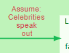
The other no-parent Variables in the diagram are not under our control. In this example, they have also been expressed as Statements (“Celebrities speak out” – rather than not speaking out.) The difference made to the downstream variables such as “Legislators have more favourable views” take these Statements or assumptions into account.
Use “♥” for Variables we value, or “☹” for Variables we don’t
In many Theories, the “no-child” Variables (the ones with no consequence Variables) are all assumed to be ones we care about (and the only ones we care about).
But of course the world isn’t like that.
Sometimes it can be really useful to show which Variables we value, e.g. by marking them with a heart ♥. (We can also use a “frowny” symbol: 🙁 for things we don’t want.)

In this case, we value the legislators and the public having a more positive attitude to same-sex marriage not only because they are more likely to pass the law, but for other reasons we aren’t mentioning here.
It’s also possible to write more than one symbol, for example: ♥ ♥ ♥, to distinguish, say, between things we value a little and which we value a lot. Or just write e.g. “Value=high” or “Value=low”.
What makes a Theory into a Theory of Change?
A Theory of Change is someone’s Theory about how to get something they want by intervening on something they can control.
A school Principal has this Theory …

So this is a Theory of Change (for the Principal):
- she believes the Theory
- she values at least one Variable
- she controls at least one Variable
Theorymaker symbols:
► = we can control this
♥ = we value this

This example happens to include just three Variables in a chain-like structure. Countless other structures are possible.
Listing assumptions on the arrows
Text added to an arrow, preceded by the word “Assumption:” or “Assume:”, shows that there is actually an additional influencing Variable. This is just an abbreviation: it saves space rather than having to actually add the additional Variable to the diagram.

This Theory is fine, but we can also simplify it …
… like this:

An “assumption”, expressed like this, is nearly always a “false, true” Variable like “Celebrities speak out” rather than, say, a continuous Variable (like “How much celebrities speak out”). ℹAlso, we probably imply something about the factual level of these assumption Variables - see later
Bare arrowheads for unnamed additional influences
Bare arrowheads (without any lines) are used to show that there are some other influences in our Theory of Change; we can’t, or don’t want to, specify what they are but we don’t want to forget them.

The additional green arrowheads, like here on the Variables “Law is passed” and “Public opinion improves”, remind us of the presence of other, unnamed, influences.
Showing specific features of Variables, like who (or what) they belong to, like this: “Child: …”
We can specify who or what a Variable belongs to, by mentioning the ‘owner: …’ at the start of the Variable name. We can do the same for any other feature which a Variable might have, e.g. time-point, country, county … and which might distinguish it from other Variables.)

This suggests that somehow, trust in strange dogs depends on opportunities for interaction.

Grouping boxes for Variables with similar features
When the labels of several Variables begin with the same feature or owner e.g. “Child:”, they can be surrounded by a grouping box; that text is then deleted from those Variables and added to the box. It’s the same thing, it just saves a few words and helps structure the diagram.

This Theory says that trust in strange dogs depends on opportunities for safe interaction.
Both Variables have a special feature (Child:...) which tells you who or what the Variable belongs to.
Other kinds of box are summarised later.
Deleting identical information from both Variables (the fact that they belong to the child) and transferring it to a box which groups them:

The grouping box also reminds us that these two Variables belong to the same child. That has very important practical consequences.
One Variable for each person in a group
The words “For each” at the start of a Variable label, followed by a (explicit or implicit) list of people, time-points etc., says that this is actually a set of Variables, one for each person or thing in the list.
The same teacher teaches three different students - his ability contributes to their achievement, and their achievement in turn influences his pride.

Sets of Variables like this (similar to one another but belonging to different people or time points, or countries, or firms …) are very common.
Some people, especially statisticians, use the word “variable” only for sets of Variables like these. That can make things simpler in statistics, but in Theories of Change we often have individual Variables as well as sets of them. Theorymaker suggests calling these sets “for-each Variables”: treat them like one Variable but remember, really it is a set.

“^^”: “for-each-time” Variables which repeat across time
A “^^” symbol shows that a Variable is actually a set of discrete Variables, stretching across time, e.g. across the life of a project. This kind of set is also called a “for-each-time” Variable; we draw just one though we know it actually represents several ℹThis could be a discrete set of Variables, e.g. one for each day, or, in principle at least, the “for-each-time” Variable could mark off a continuous stretch of time which we could measure at any given second or micro-second, like a patient’s temperature.
In Theories of Change, unlike in statistics, we assume (unless told otherwise) that Variables exist just once in time, e.g. a voter’s decision to vote a certain way on a particular election day with a specific date,, like this.,

Variable sets which stretch or repeat across time can be replaced with “for-each-time” Variables.
These two diagrams are equivalent. Here, the set of three Variables, one for each day, has been replaced by a single “for-each-time” Variable.

“^”, and related symbols, for individual events
A circumflex symbol (“^”) says that a Variable is defined just once, at a single point in time.
What if we need to make it clear that a particular Variable represents an individual event? These symbols can be useful:
^ = a discrete Variable which happens just once, at some time during the time period in question
^_ = a discrete Variable which happens just once, at the beginning
_^ = a discrete Variable which happens just once, at the end
We already saw ^^ for a discrete Variable which repeats many times, e.g. daily.
In this Theory, the first and third Variables take place at single time-points.ℹThe Variable in the middle is probably a “memory” Variable.

Many traditional Theories of Change are sliced into “phases” which define when the Variables within it start and end. With more flexible Theories, such as those you can make with Theorymaker, we can’t assume that a project has strict phases.ℹor that there is a “time axis” within the Theory of Change We need other ways, like these symbols, to show a Variable’s timing.
“~”: “for-each-time” Variables which stretch continuously across time
A “~” (“tilde”) symbol shows that a Variable is actually a continuous set of Variables, stretching across time, e.g. across the life of a project. This is called a “for-each-time” Variable; we draw just one though we know it actually represents very many ℹ (actually, an “infinite number”) . Continuous “for-each-time” Variables mark off a continuous stretch of time which we could measure at any given second or micro-second, like a patient’s temperature.
Continuous for-each-time Variables are distinguished from discrete ones which are marked with “^” and related symbols.

The “~” symbol in the intermediate Variable below shows that trainee skills are conceived of as stretching right from the beginning to the end of the project. You could test a trainee any time you choose. (The first Variable only makes sense at the beginning of the project and the last one only makes sense at the end).

Dashed arrows: for defining Variables in terms of others
Dashed arrows pointing to a Variable show that it is defined in terms of the Variables at the beginning of the arrows, not caused by them.

The arrows in a Theory of Change should show causal influence. But the last Variable above is just the sum of the other two, ℹAssuming there are just two Regions in the country by definition - so we should use dashed arrows:

Where necessary, you should specify the function involved – in this case, logical AND.
Or omit the defined Variable completely and group your Variables visually using a box:

Note that where we had a “mathematical” function underlying the causal influence, we have “mathematical” function underlying definitions. The two cases are exactly parallel.
Dashed borders: for Variables which are defined in terms of others
A dashed border around a Variable shows that the Variable cannot be independently measured because it is defined in terms of others. So if you’re planning to count the number of girls and the number of boys, it doesn’t make sense to also ask for the number of children as if it was additional information.ℹDashed lines can be used too. .
We already saw that to include a defined Variable in your Theory, you can use dashed arrows. But here, we have also added a dashed border around the last Variable.

Again, where necessary, you should specify the function involved – in this case, logical AND.
If you already have “indicators” for the defining Variables, there is no need to seek additional “indicators” for the defined Variable as well. The evidence is shared.ℹBut this Variable is just as real as the others. Definition and causation are about relationships, not Variables.
Combining contexts
The context in which a particular Theory applies is the intersection of the contexts of all its constituent bits.

… and this theory is valid only for children …

… giving a new Theory which is valid only in the context which is the intersection of the two contributing contexts: male children.

ℹ If even one Variable in your Theory has a fixed time, they all do. foot-
SECTION 4: Different kinds of influence
This section (work in progress) is about the kinds of influence which Variables can have on one another: how and how much. We encounter words like “linear”, “necessary” and “interaction”.


Problem: Specifying the kinds of influence between Variables

This simple Theory tells us that some Variable(s) influence another, but we want to know how: what level of the consequence Variable to expect for every combination of the levels of the Variable(s) which influence it? However, this seems like a hopeless task. For one thing, most social scientists assume that the causal connections must have the form of precise numerical functions - even when we only have imperfect knowledge of them.
Maybe student satisfaction = student's feeling of living up to expectations. This describes a linear relationship. But why should the relationship be linear? There are uncountably many possible functions from a numerical Variable to another. Will we ever have enough information (or time) to establish a really robust theory about the exact shape of this function? And what happens when we have more than one influence Variable? The (arbitrarily complicated) function from living up to expectations to student satisfaction might be different for every different level of some additional influence Variable. A real Theory of Change is composed of many such simple Theories; are we really supposed to identify (or carry out ourselves) serious research which gives us precise formulations of each of these functions? No, we don’t have the time or money.
As evaluators, we need:
- serious, clearly-defined ways to roughly specify the influences which Variables have on one another, (like “frustration increases as stress increases”)
- rules for doing “soft calculations” with such statements,
- rules for roughly working out “effect”, “contribution” and “impact” based on a Theory and some data
- and we need all this to work for all the different kinds of Variable (and influences between them) which we are likely to encounter in Theories of Change.
⊕: “Plus” influences
A “plus" symbol ("⊕") on an arrow from A to B means that any increase in A will lead to an increase, or at least no decrease, in B. ℹ And we specify that A has to have some effect on B, i.e. the influence of A on B is not completely flat. Most influences in real-life Theories of Change are”plus". In Theorymaker, we assume that if the type of influence is not specified, assume it is “plus”. So normally, we only bother with the ⊕ symbol when we need it to avoid ambiguity. ℹ Plus, maybe there is an implication that any likely Difference on the influence Variable will lead to a Difference on the consequence Variable which has practical significance . Otherwise, we should only use a thin arrow.
How warm you feel depends partly on the strength of the sun. These two diagrams are equivalent; in the second, the “plus” symbol is used instead of words.


These are usually called “positive” rather than “plus” influences, but that is confusing when the consequence Variable has negative valence, e.g. what is a “positive influence on mortality”? That’s why we prefer the word “plus” in Theorymaker.
“Plus” influences can be specified between any directed Variables - that’s a majority of Variables in real-life Theories of Change, including “false/true” Variables. They are essentially what a mathematician would call “positive monotonic functions”.
“Plus” is just the Theorymaker word for “positive monotonic” in maths.
⊖: “Minus” influences

This arrow could be misleading because strength of wind makes us feel colder, not hotter.
We prefer to refer to “plus” and “minus” influences rather than “positive” and “negative” influences, because the latter can be misleading when referring to Variables which we don’t like - for example, what is a “positive influence on mortality”?
Theorymaker uses a blue arrow and/or a ⊖ symbol to mark minus influences: any increase in wind means a decrease in subjective temperature.

Minus influences work with false/true Variables too, just as plus influences do.
“Plus” (or “Minus”) influences with false/true Variables
As “plus” (and “minus”) influences are defined on any directed Variables, in particular they work for “false/true” Variables.

If we conceive of wearing warm clothes as a false/true Variable, in the right circumstances, you will feel warmer when you are wearing warm clothes, other things being equal. So this is a “plus” influence of a false/true Variable on a lo-hi Variable.
Later we will look at the influence of two or more false/true Variables on a false/true consequence Variable.

If we also conceive of sweating (as well as wearing warm clothes) as a false/true Variable, increasing the sunshine (in the right circumstances) leads to sweating. So this is a “plus” influence of a lo-hi Variable on a false/true Variable.

If we conceive of both as false/true Variables, then in the right circumstances, you’ll sweat if and only if you are wearing warm clothes. Some real-life Theories of Change consist only of these kinds of Variables.
A “plus” influence is probably not linear

The “⊕” symbol tells us that the influence of support for the law among the population is “plus”, i.e. an increase in one leads to an increase in the other. But is this influence linear (e.g. a 1% increase in population support means that support among legislators always goes up by a fixed amount, say, 2%)?
A linear influence
And what if we can’t even agree how to measure or express the Variables in terms of numbers? ℹ It seems quite natural to draw a rough graph to illustrate plus influences. But if these are only lo-hi Variables, drawing graphs suggests a level of measurement (interval or ratio) which we don’t have - see (Stevens 1946). So we have to be careful how to interpret them. We musn’t get tempted to say, for example, that two pairs of points are the “same distance” apart. For instance, linear influences can’t even be properly defined for lo-hi Variables (so we can’t really even draw graphs either).
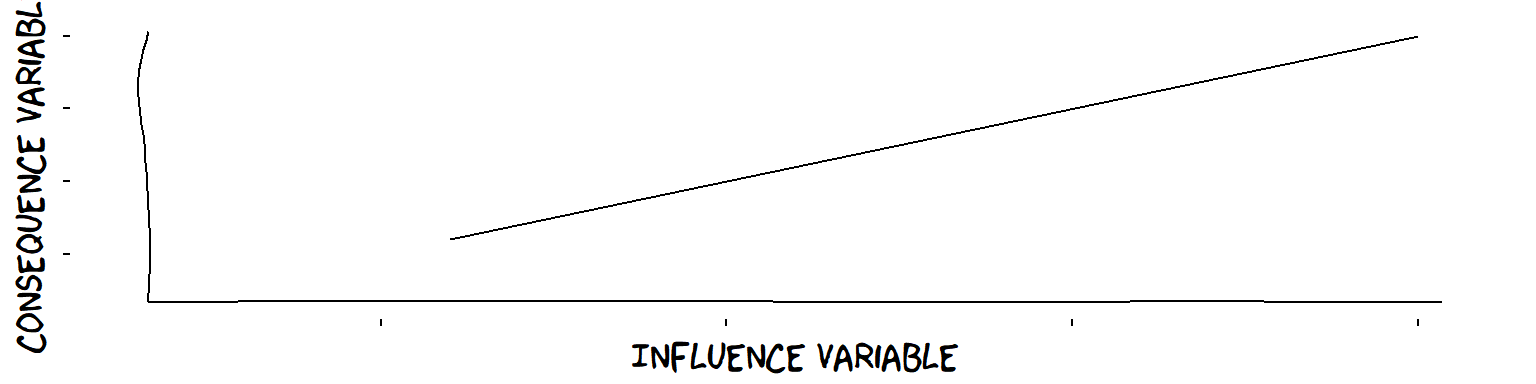
Well, Theorymaker argues that the idea of a “plus” influence is much clearer and more universal than the idea of a linear influence. “More of this means more of that” is pretty easy to understand and not impossible to verify. Real-life Theories of Change are full of plus influences.
A plus influence
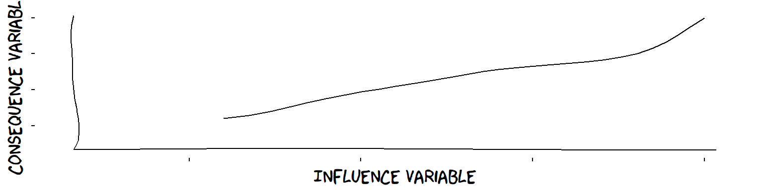
Not a plus influence, because of descending section
All of this applies to “minus” influences too.
Special kinds of “plus” influence with just one influence Variable
- S-influences (from continuous Variable to continuous Variable) ℹWhen all the members of a set of more than one influence Variables (independently) have plus influences on a lo-hi Variable, the influences are probably S-shaped. This is the equivalent of linear superposition amongst interval Variables. For example, characteristics of parenting style and size of apartment and IQ at age 10 might all have a plus influence on happiness at age 25. If happiness is scaled from, say, 0 to 100, then these influences must gradually decrease as happiness increases, otherwise we would break the ceiling of 100.
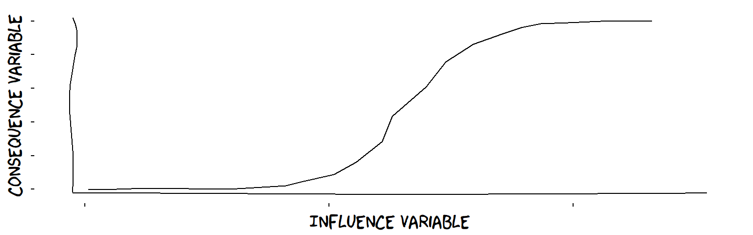
An S-shaped influence
- Threshold influences (from continuous Variable to continuous Variable) …
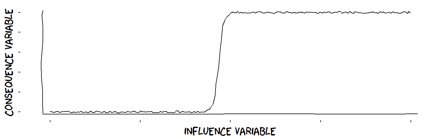
A threshold influence
- Threshold influences (from continuous Variable to false/true Variable) …
…
- Increasing influences
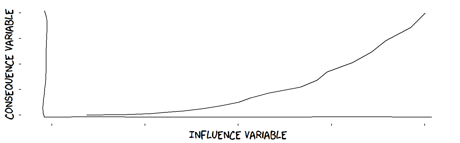
An increasing influence
- Decreasing influences
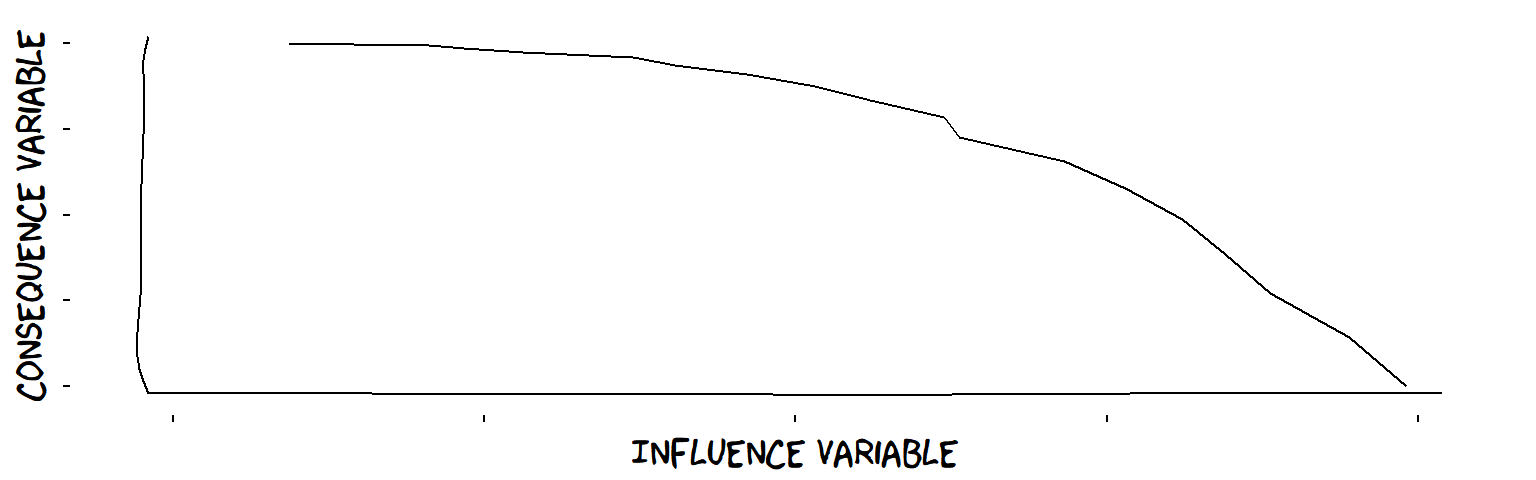
A decreasing influence
For each of these, there is a parallel for “minus” influences too.
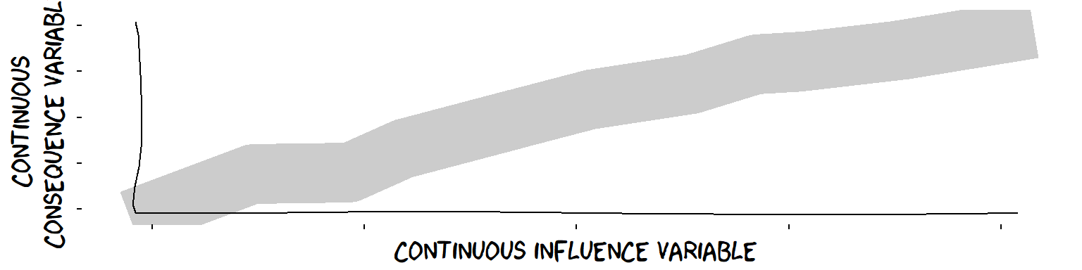
We can also emphasise uncertainty around the consequence Variable by showing a band rather than a line
Influences which are not “plus” or “minus”
“Plus” (and “minus”) influences are a very wide class which cover very many of cases we see in real-life Theory diagrams. But it is worth mentioning a few which are not.
- U-shaped influences
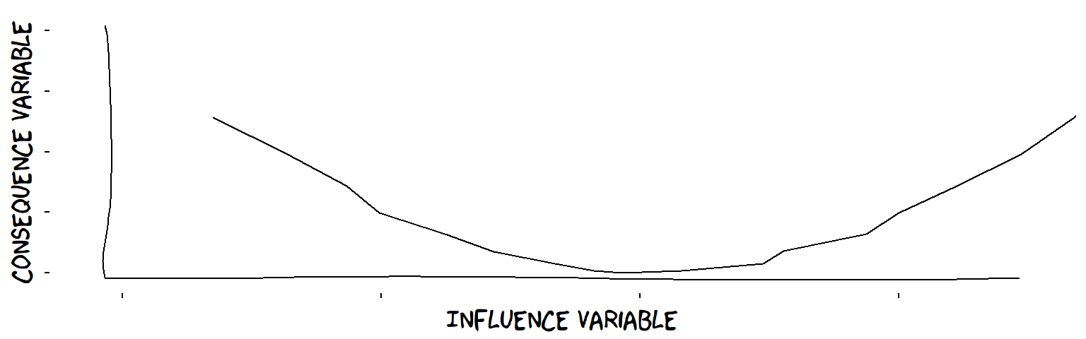
A U-shaped influence
- Inverted-U influences
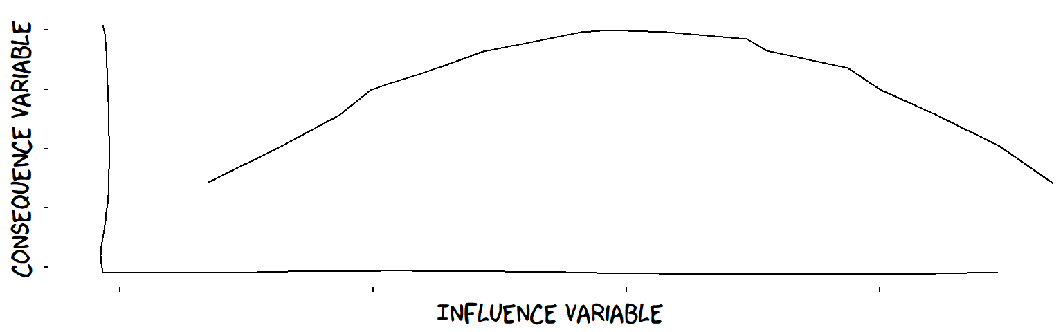
An inverted-U influence
Example: student performance in relation to level of pressure (not too much, not too little).
More than one influence Variable
We already saw that a simple Theory tells us what level of the consequence Variable to expect for every combination of the levels of the influence Variable(s).

In general, the influence of, say, feeling supported and liked might be different for every different level of living up to expectations.
A very confusing interaction between a continuous influence Variable and a discrete influence Variable
Independent influences
If a set of Variables have independent influences on a consequence Variable, this means that the influence of each Variable is completely unaffected by the levels of the others. ℹ The influences of independent interval Variables can be literally added up. This is called “linear superposition” and is part of what people mean when they use the word “linear” when talking about Theories of Change.
Assuming independence makes life easier because we can break down their collective influence into separate influences, one for each Variable, which work independently, of one another. This is simpler to think about and work with. However, it’s a big assumption which is nearly always false!
There are easier ways of thinking about issues like independence – see next slide.
When people talk about linear influences in Theories of Change, they often mean the idea that, if a Variable has more than one Variable influencing it, the total influence on it is just the sum of the influences of the individual influence Variables. In other words, to know the influence of “Support among population” on “Support among legislators”, it is not necessary to know anything about “Pressure from party leadership”, and vice versa.
“Linear” in this sense is short for “Linear superposition”. Quantitative scientists like it because it makes things easier to calculate. But it would be “fake science” to think that therefore, that’s how the world is. Suppose for example that, when interpreting support from the population, individual legislators consider what the party leadership thinks. For example, if the leadership is totally against, pressure from the population might have a negative influence on legislators.
“Robust influences” - a rough way to talk about “independence”
An influence on a consequence Variable is “robust” if the type of influence (“plus”, “minus” etc.) does not change when the levels of the other influencing Variables change. ℹ So the other Variable(s) might affect the fine detail of the influence but they don’t change its original type. This means that whether an influence counts as “robust” can depend on how it is characterised. So an influence which is characterised as “plus” might be robust, but if it was characterised as “additive” it might not be, because characterising an influence as strictly additive is stricter. It is less likely to remain additive at every level of the other influence variables. Influences which are specified as numerical functions - for example linear, exponential, etc., are only separated if they are actually independent.
This is a much more realistic assumption than actual independence; much more likely to actually happen in real life. We mark a robust influence on the individual arrow. If an influence is, say, overall plus but not for every level of the other influencing Variable(s), we can mark it on the arrow but add a “?”.

So in this case, the influence of the wind on subjective temperature might be affected somehow by the strength of the sunshine, but it remains “minus” whatever the sunshine (and the influence of the sunshine is “plus” regardless of the wind): the influences are shown on the arrows.
Wind strength certainly affects the influence of sunshine on temperature; they are not “independent”. But, for each level of wind strength, the influence of sunshine remains “plus”, so we can say that "the ‘plus’ influence of sun and the ‘minus’ influence of wind are both ‘robust’.
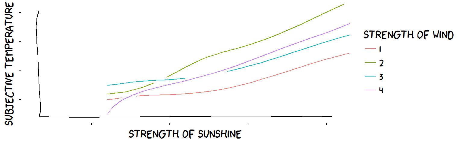
The two influence Variables are not strictly independent but they are ‘Robustust’ when characterised as ‘plus’ and ‘minus’ influences
Influence symbols in Variable labels
An influence symbol in a Variable label (rather than on the arrows) says that all the influences are of this type (and are ‘robust’).


Using “?” to show that an overall influence is not robust
If one influence on a Variable when ignoring or aggregating its other influences Variables is, say, “plus”, we can say that it is “overall plus”; and if it is not robust, because the influence is not always plus for some levels of the other influences, we can mark it on the arrow but with a “?”.
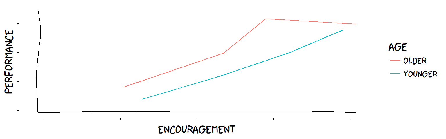
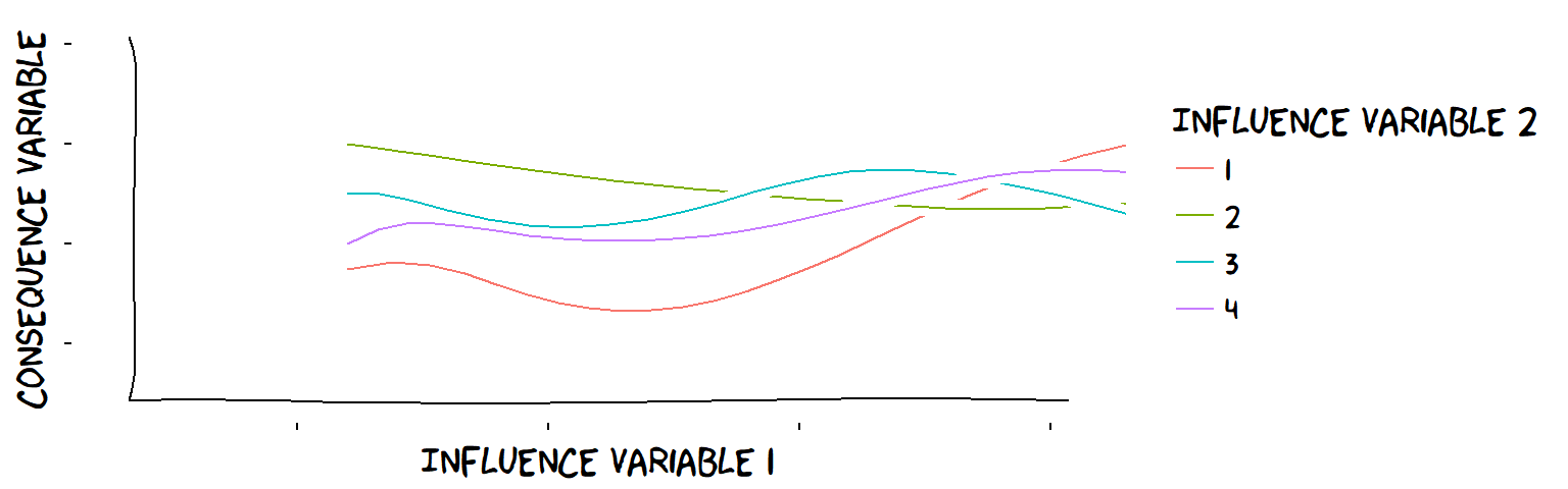
The influence of encouragement and age on children’s performance on some task
Overall, the influence of encouragement on the children is plus ℹ This is made-up data, as usual! , but not robust: for one age group, increasing the level of encouragement does not always bring increases in performance (older children respond poorly to too much encouragement).
This is information which is practically useful. It means, before you considered age, you could adopt the overall rule (“more encouragement is always good”). When you enriched your theory to include the age groups, you realised you had to consider the child’s age when applying this rule.
The influence of age, on the other hand, is plus, and robust (older children always score better, regardless of the amount of encouragement). If the blue line had crossed the red line, the influence of age would not have been robust, and we would have to add a “?” to the other symbol too.

Combined influences: Joined arrowheads

Individually, number of staff and quality of management both have a positive (plus) influence on the success of the intervention. But if the management is poor, adding staff can actually make things worse, i.e. the influence of staff number is no longer plus, and the success is endangered. We say that the influences are not robust and the arrowheads are drawn joined.
We should explain more about this lack of “robustness” in the diagram or the narrative, so the reader has a rough idea of what the different combinations of the influencing Variables does to the consequence Variable.
Combined influences: synergy

These influences are all plus, and they are robust because, for each Variable, whatever levels the other Variables have, its influence on the consequence Variable is still “plus”.
But, often we assume a kind of synergy: that the total influence of one Variable on the consequence Variable always gets larger as any of the other Variables increases. We can call this “synergy” - a subtype of multiple, separate, plus influences. ℹ But how coherent is this idea really? If the consequence Variable is lo-hi, the influences have to drop off asymptotically at some point. And, should we draw the arrowheads separate or together?

Combined influences: maximum and minimum
An influence which is the maximum of two Variables
An influence which is the minimum of two Variables
A very interesting special case is when all three Variables are false/true.
Combined influences: two false/true Variables (necessary & sufficient conditions)
When we have two (or more) false/true Variables influencing a false/true consequence Variable, there are not many different combinations. We find that if both are “plus” and/or “minus”, the influences cannot be robust. There is always a kind of dependence.

The influence of Spark on Fire is plus, and likewise for Oxygen. But both are necessary, so if one is absent, the other is no longer plus: these influences are not robust. We draw the arrowheads together and write “AND”.

The influence of either flamethrower is plus. But both are sufficient, so if one is present, the other is no longer plus: these influences are not robust. We draw the arrowheads together and write “OR”.
We can think of AND and OR as a special case of, more generally, “maximum” and “minimum” combinations of influence Variables.
See also INUS condutions.
Delays
Generally, influences between Variables with a relative or absolute time should have a delay specified with “Delay: ” - in general on the consequence Variable, or on the arrow if the influence is robust. The delay specifies how much later is the consequence than the influencing Variable (this is not necessary if relative or absolute time is already specified on the Variables). This is necessary also in the case of repeated or continuous Variables.

Specifying delays between repeated and continuous Variables can be quite challenging:

Feedback loops
If you can follow the arrows from one Variable back to itself, the path is called a “feedback loop”.ℹBasically all the causal networks in Theorymaker are really DAGs - Directed Acyclic Graphs (Pearl 2000) . Loops are only possible with for-each-time Variables, which are actually sets of Variables, so there is no actual loop from a Variable at a single time-point to itself, otherwise it would be causing itself.

The Variables involved must stretch across time; the “~” in front of a Variable name shows this. (The ↺ symbol is explained later.) Variables with a fixed time-point, common in very simple step-by-step Theories such as most “logic models” can’t take part in a feedback loop.
The delay may need to be specified if not obvious.
🞕: Influences which “optimise” the level of the consequence Variable (in feedback loops)

Here, program staff know the volunteers are most effective at a medium level of excitement, so if the volunteers are too lethargic, they offer plenty of inspirational input and if they are too excited, they try to calm them down.
We use the Theorymaker symbol 🞕 to show that the influence which controls the Level of a Variable in a feedback loop is aimed at maintaining some kind of optimum, pushing up low values but bringing down high ones. It is unlikely to be a simple “plus” influence aka “positive feedback”. Why not?
↺: “Memory” Variables
How does sea temperature depend on sunshine?

(The ~ sign says this Variable repeats continuously across time.)
… but this suggests that the sea temperature plummets every time the sun goes behind a cloud.
In fact the sea takes a long time to cool much: to know its temperature at one moment, we need to know about sunshine and the temperature in previous moments: it’s a “memory” or “stock” Variable.

An arrow from a Variable to itself or a ↺ symbol in the body of the Variable indicate a memory Variable: one whose level depends partly on its own previous level.

!flow: “Flow” configurations with “Valve” Variables
A “!flow” symbol on a grey arrow from X to Y with a tapering arrow incoming from another Variable V, can be understood as a “Flow” configuration, simulating the way that material flows from X to Y under the control of the “valve” Variable V.
This can be translated into a pair of more basic Theorymaker concepts: an “Upstream” influence on the upstream Variable and a “Downstream” influence on the downstream Variable.

Here, the arrows do not represent causal relations but are like pipes for transferring material, as if the apples actually flow down those pipes. The diamond shapes represent “flow” or “valve” variables. You can imagine they could be just closed or open, or limit flow to a certain amount. (These kinds of elements are central to “stock-and-flow” diagrams which are familiar from Systems Dynamics. ℹ (The oval shape at the start is called a “stock” and the final oval shape a “sink”.) The arrows are sometimes drawn as double lines.)
The direction of the arrows are like the direction of gravity; when the valves open, the apples flow, and the wider they open, the faster the apples flow. So the green variables are measured in numbers of apples, whereas the flow variables are measured in apples per minute.
It is possible to reproduce idea of flow in Theorymaker. Here is how the stage from warehouse to shop ℹ (the others are simpler) is represented using more basic Theorymaker elements; all we need to do is clarify what the “upstream” and “downstream” influences are. They are explained if you hover over the “Fundamentals” button above.

So we have succeeded in translating a flow of material in terms of basic Theorymaker elements using only our more fundamental concept of causation. ℹ Real-life “stock-and-flow” diagrams usually include information links as well. These are no different from normal Theorymaker arrows and so need no special treatment. When combining these ideas to translate larger diagrams such as the one on the left, the levels of the intermediate Variables (Warehouse and Shop) are determined by two influences - a Downstream influence as the recipient of apples and an Upstream influence as the source of apples for the next Variable.
Definitions of the pair of “Upstream” and “Downstream” influences which we need to model stock-and-flow diagrams.
\[Upstream(V,W_{t1})=max(W_{t0}-V,0)\]
So if, for example, time is being measured in seconds and flow Variable V is being measured in apples per second, you can calculate the level of apples in the upstream container W (“Warehouse”) by using this Upstream function: the level will be the level of W in the previous second, minus V, unless the level of W in the previous second was 0, in which case the level of W now will also be zero - because we have run out of apples and we can’t have a negative number of apples.
\[Downstream(V,S_{t1},W_{t0})=S_{t0}+min(V,W_{t0})\]
Similarly the level of apples in the downstream container S (“Shop”) can be calculated by using this Downstream function, which also depends on the upstream Variable - because the level of S will be the level of S in the previous second, plus either V, or the number of apples left in W in the previous second if this is less than V.
“Source” and “Sink” Variables - the first and last in the chain - are trivial; their levels are always “infinity”, so they never change and we don’t need to bother calculating them.
These definitions only deal with discrete time. To deal with continuous time, one would have to generalise these functions.
The case of the camel’s back: a memory influence leads to a threshold influence
A camel’s back is a combination of a memory influence followed by a threshold influence

There are plenty of real-life instantiations of this kind of causal chain.
Good practice: Noting the evidence for specific influences, on the arrows

In this diagram, the evidence for the collective influence of both Variables has been added to the “influence” part of the consequence Variable’s label. And an additional piece of research which supports the influence of just one consequence Variable has been noted on its arrow.
See also Dunford’s suggestion to use arrow colours to represent the strength of evidence (Dunford 2012).
Thicker arrows for bigger influences
The thickness of the arrows in a Theory of Change can be used to show the relative strength of the corresponding influences.ℹThis assumes that we can actually say or calculate what the relative strength of the influences are, see later.
Here, we want to show that the influence of the other campaign is much less important than public opinion.

We can do the same thing with the sizes of bare arrowheads for unnamed influences.

Here, we want to show that the other influences on public opinion are much more important than our campaign; and that the other influences on the legislators are relatively insignificant.
Do we assume that, if not otherwise specified, the presence of a normal-sized arrow on a diagram means that the size of the influence is not just tiny but of practical significance?
Grouping boxes to organise projects
In general, a diagram in which several Variables have the same text as part of their labels is equivalent to one in which those Variables have the text removed from their label but they are surrounded by a grouping box with that text as its label. This can be useful e.g. to organise projects, to group Variables into sectors, phases, sub-projects, regions etc.

Arrows from grouping boxes

We often see this kind of diagram in the wild.
An Arrow from a Box is usually a kind of a shorthand which replaces Arrows from the Variables it contains…
… so it is equivalent to something like this:

… but … Are the influences supposed to be “plus”? How do they combine - are they all “robust”? Perhaps one or two of the Variables in the box have no influence? Perhaps the Variables in the box combine into one single Variable which then influences the consequence Variable?
The minimal interpetation is this:
An arrow from a box to a Variable V means that at least some of the Variables in the box have some kind of influence on V.
Arrows to grouping boxes

An Arrow to a Box is usually a kind of a shorthand which replaces Arrows to the Variables it contains…
… so it is equivalent to something like this:

Arrows between grouping boxes

An Arrow between boxes is usually a kind of a shorthand, perhaps just to avoid drawing too many arrows …
… so it is equivalent to something like this:

… but … are these supposed to be “plus” influences, or what? Were all the possible arrows really implied? Are the Variables in the first box combined before influencing the Variables in the second?
The minimal interpetation is this:
An arrow between boxes means that at least some of the Variables in the first box influence at least some of the Variables in the second, in some way.
A Theory of Change can have more than one valued Variable

Lots of Theories of Change have only one valued Variable,
- the last one in the chain
- often called “Top-level Outcome”, “Goal” etc.
But in the real world, you (or maybe other stakeholders) often value more than one Variable.
The laptops might have other valuable consequences for the students, so mark them as valuable, e.g. “♥” or even “♥ ♥”.

Intemediate Variables can be valuable too

In the real world, you (or maybe other stakeholders) might value Variables which are not at the end of a chain. If so, mark them as valued too, e.g. with a " ♥".
Maybe you would still be quite pleased with the project if it made a big difference to student self-confidence regardless of its effect on exam results:

Some intermediate Variables (like attending workshops) are really only means to an end.
But some are valuable in their own right: don’t undersell your project if it really does produce additional value! Add more " ♥" for Variables you value more!
Intrinsic value

We already noted that a valued Variable does not have to be at the end of a causal chain. In fact, it can even be at the beginning of one.
This kind of thinking is very important for instance to understand spiritual and religious motivation. It is related also to the idea of the “humanitarian imperative”. From this point of view, the consequences can be more or less important, but certainly the process is important.
Multiple Actors: Who acts on what, who values what?

When different stakeholders or “Actors” interact, they are usually able to intervene on different Variables. This can be done by using different colours, or by writing the name of the Actor before the ▶ symbol, as we do here. We can use ♥ symbols, preceded by the name of the Actor who values this particular Variable, in the same way. ℹ♥ symbols are only assigned to stakeholders who are also actors - because only they can change anything?
Previously we have only seen Value ♥ and Control ▶ symbols used globally to show what “we”, the makers of the Theory, value and control. Now we are zooming out and taking a meta-perspective.
This kind of presentation can be really useful for realising that different Actors might do different things, or put different a different emphasis on the same things, because their motivations are different.
In this example, part of the trainer’s motivation is simply the act itself - of providing pro-bono training. All the Actors value the main outcome, improved teaching, whereas the increased pay to which the teacher is entitled after completing the training is a positive motivation for the teacher but a negative one for the Ministry. ℹ A later slide expands on this one, focusing on the fact that not just one but several teachers might be involved.
In this case, the Actors differ on two of the dimensions of the Theory of Change - what they control and what they value - but share the third aspect, namely the Theory itself, the one shown here. More generally, they might not.
See also (Hansen and Vedung 2010) on evaluation with multiple stakeholders, and (Van Ongevalle et al. 2012) for “actor-focused” evaluation approaches.
Re-evaluating value

Michael Scriven is one thinker who has often raised the question of which values are really valuable, and encouraged evaluators to (re-)evaluate officially posited values.
In the diagram, the two intermediate Variables, the planned Outcome and another interesting Outcome (which may or may not have been planned) are assessed in terms of value above and beyond the value expressed in the one Variable which was originally posited as being valuable (“♥”). The rules about how to assess them in terms of shared values, and indeed the shared values themselves, are marked here (spiral symbols) as inter-subjective: we can hopefully agree on them in retrospect but we can’t definitively specify them in advance.
Interestingly Chen & Rossi’s original paper (1980) on Theory-Based Evaluation focuses also on multiple goals ℹ(they say, why not include all the Variables which might be affected by the program, in the opinion of different stakeholders; why not assess value for each of different subgroups …) and the possibility of re-assessing originally posited goals.
FundamentalsOf course, merely drawing a picture tells us nothing about how this is actually to be accomplished in an evaluation. But if indeed values are not in the end distinguishable from facts, we shouldn’t necessarily need completely new methods.
SECTION 7: Effect and contribution: Doing calculations with Differences
This section (work in progress) is about how to calculate the contribution of some Variables on others.
We encounter words like “contribution”, “attribution”, “effect” and “impact”.
Statements: using double brackets and _ to report the actual (or “factual”) level of a Variable
All of these are Statements:
The last three examples give (optional) specifications of levels; two use symbols and the last one gives an explicit list.
The trailing "_" helps to distinguish Statements from Differences and also from summarised Differences.
These Statements are more or less equivalent to ordinary English sentences - the kind of sentence which can be right or wrong. But they use double-brackets to make clearer than ordinary English does which is the part which could be different. We can write them just as sentences or we can also include them in graphical Theories of Change.

This very simple Theory tells us that the opinion of the constituents might have some kind of influence on the passing of the law; and it also tells us that the support level was about 50% and that the law was actually passed. But the diagram doesn’t give any indication whether the law would have been passed had the level of support been lower, or even higher - so actually it isn’t much use to us as evaluators or managers.
If you compare the trailing “" in a Statement with how a Difference is formulated, you can imagine that the counterfactual level which would make this into a Difference, which could go after the "” or the “rather_than”, is missing.
Statements on their own are not enough to establish causation.
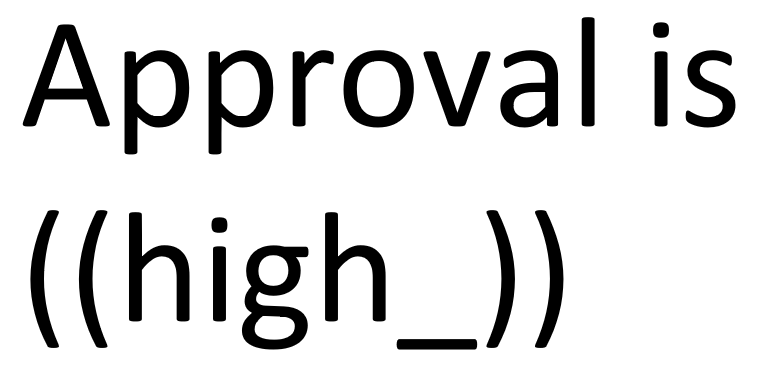
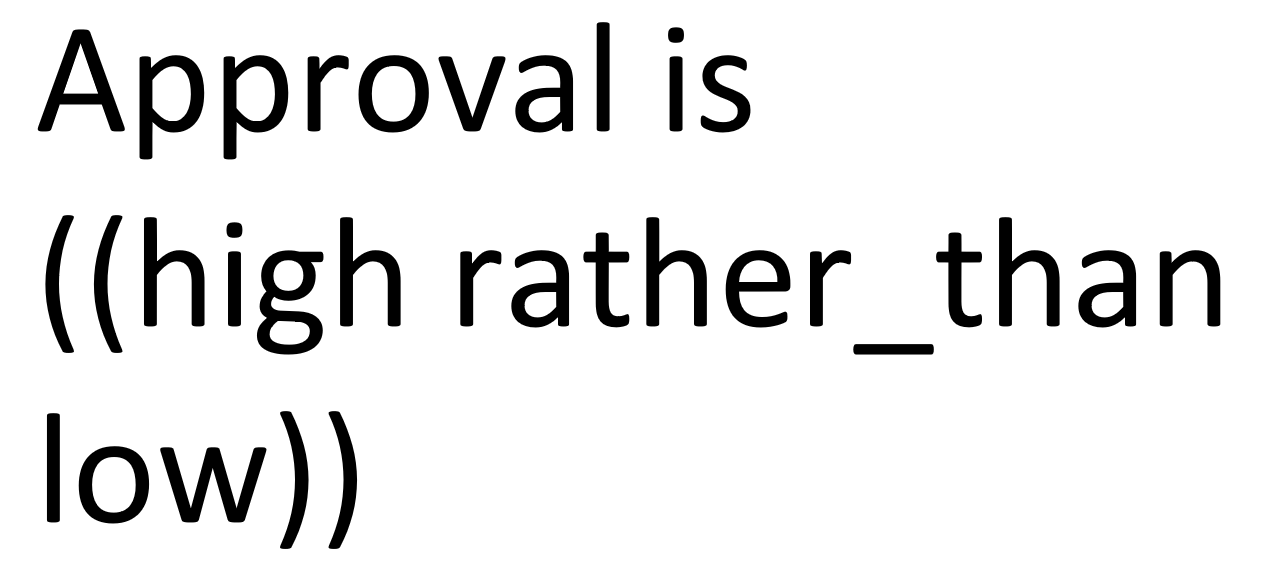
Differences: the Variable takes its factual level “rather_than” the counterfactual level, expressed within double brackets
Formulations like “Approval rating ((very good rather_than poor))” are called “Differences” - with a capital D. Meaning: the approval rating is very good, (rather than poor, which is perhaps what we were expecting).
When something happens to a Variable, e.g. we change its Level deliberately, its factual level becomes something different from what we otherwise expected (“the counterfactual”). So if we decide to stock up a food warehouse which has only 100kg of food with another 500kg, we can say:
As binary Variables have only two Levels, a Statement about it is equivalent to a Difference. So this “Difference” …
… says that the Prime Minister agrees (rather than not agreeing), and so does this “Statement”:
A Statement does not contrast the actual (“factual”) level with any counterfactual (expected or background) Level.
The distinction between Statements and Differences is clearer with non-binary Variables, especially when they are joined up into Theories.
I’d argue that it is only possible to make causal claims using Differences. And I wouldn’t stop there: I’d argue also that a causal claim only ever makes sense within a Theory - whether that Theory is explicit or implicit.
A Difference is a like subtraction, but more general. If the Levels are numbers, we can often actually do subtraction to express the Difference as a single number.
Differences are the basic currency of Theories and Theories of Change. Understanding them is key to understanding how we can make claims about causation.

Whereas this tells us that the MP voted for the law rather than against because 50% rather than only 30% were in favour. Had the level of support been 30% or lower, the MP would not have voted for the law; but 50% was more than persuasive.

✔,✘: Ticks and crosses for affirmative and negative Statements
“✔” means that this is a false/true Variable which is also asserted to be true, i.e. to take its true level rather than its false level. “✘” means that this is a false/true Variable which is also asserted to be false, i.e. to take its false level rather than its true level.
We already saw that there are different ways to express positive (and negative) Statements in Theorymaker.
Here is the canonical way:
These are very useful when we look at causal networks containing false/true Variables.
They are also very useful to show when binary events happened or didn’t happen when looking at a project plan retrospectively.

In this case, only the planned lobbying of Party A was actually carried out, but this was enough to convince their representatives and so the law was actually passed.
Targets imply specific influences between the Variables
NGO financial resources ((increased by 1000 EUR)) - this leads to ((extra)) teacher training weekends, which leads to ((an increase of 20%)) in teaching quality.

Often, we don’t try to show the nature of the influences in our Theories, and perhaps claim not to even have thought about them. But we are very happy to set targets on Variables downstream from our interventions - and to be able to claim such downstream influences we are implicitly claiming a lot about the strength and nature of the influences (… a Difference of 2 training sessions here is enough to increase teaching quality by 20% … ). In this case, the reader can work backwards from the targets to get a rough idea of what influences are implied. (Evidence?) ℹ Problem of attenuation.
Actually, setting targets in this way is probably quite a good way to specify the size and nature of influences.
Making claims about contribution

Actor of this ToC claims:
- control over quality of teacher training, will improve it by 50%
- this leads to a 20% improvement in teaching quality & then to a 10% improvement in student achievement
.. but knows there are other influences, control is incomplete


Soft arithmetic

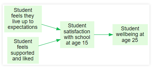
In this diagram, the influences are both specified as “plus”: any positive increase on the influence Variable makes a positive increase on the consequence Variable: when a student feels that they live up to expectations, their overall satisfaction with school is higher, and so on.
We might not know much about how, or what the effect will be on each individual child. We might not be able to say how much better they will feel, in fact we might not even agree in detail about how to conceptualise or measure their feeling in numbers. But Theories even with such imprecisely-defined influences can be really useful. “Plus influences” are one of Theorymaker’s ways to help present, discuss and even do calculations with roughly-described Theories of Change. Knowing there is a “plus” influence isn’t a lot of information, but it’s a lot better than none.
A first rule of Soft Arithmetic: we can deduce in this case that the (indirect) influence ofStudent living up to expectations on Student behaves positively at school is also a “plus” influence. Fundamentals
We won’t bother with a formal proof here, but it should be trivial.
Defining iterative theories in Theorymaker
An iterative Theory is one in which Variables (and the influences between them) are identified by subscripting on one or more dimensions, one of which can be thought of as time.

This is a basic example based on the work of Stephen Wolfram (2002) in which four rules are used to define the state of cells in one row of a grid based on the states of the cells immediately above and above-left of any given cell. The Variables are not defined uniquely but only relative to other Variables. The symbols on the arrows can be interpreted as “below-right” and “below”.
These kinds of iterative games have a long history - perhaps Turing Machines were the first. The point of including them within Theorymaker is that we can apply the same definitions of influence, effect etc which we have already developed to the massively extended universe of Theories which iteration allows us to navigate. For example, even quite simple rules can produce unpredictable results.
֍: Wildcard Variables and influences

We can agree what counts as evidence for “Support given to innovation at Universities in Croatia” - for example we could check lecture content - and for “Universities in Croatia are more successful” - for example, difference made to numbers of students graduating, quality of research published etc. But what about the intervening Variable?
The ֍ symbol is an emergent Variable: - given the Variable label (“More innovation at Universities in Croatia”) - we find it hard to describe in advance what evidence for it would look like - but we can mostly recognise evidence for it once we see it.
We can’t specify “innovation” very clearly in advance because if we could, it wouldn’t be innovation. So we use this “wildcard”.
!multi: “Composite” variables
The !multi symbol is used for Variables which can be understood as composed of several component Variables, all of which are ordered.

A student’s success at school, conceived here as a single Variable, certainly depends on their personality as well as other things. Here we assume that “personality” can be deconstructed into a number of component ordered Variables, indeed there has been quite an industry around that endeavour (“big five” personality dimensions, etc.). However here we are conceiving of “personality” as a single, composite Variable. The nature of the influence is probably quite complicated and so is marked with a “?” symbol.
This definition leaves open the question of whether there is a specific algorithm which defines how to combine the ordered dimensions or whether this is left open as a kind of wildcard.
;: “Rich” variables
The
; symbol is used for Variables which cover a broad range of behaviour, consequences, etc., falling under a broad label, and not just a specific measurable dimension or dimensions. Rich Variables are not usually ordered.
This scientific-seeming Theory of Change does not use rich Variables. Note that the influence of the amount of training on student academic achievement is only via the extent to which teachers use creative techniques - not even the quantity and quality, which would be a composite Variable but just the extent - a single, ordered Variable.


Subtle difference: now the intermediate Variable is a “rich” Variable which includes all and any aspects of teacher behaviour - not just the amount of creative techniques, even if we add their quality. Of course in practice we are probably interested only in those aspects which are a relevant part of the causal path from the training to student achievement. So marking a Variable as “rich” is a bit like adding to the original “poor” Variable a wildcard Variable which captures any and all other aspects of teacher behaviour in the classroom.
Most Theories of Change in the wild use rich Variables. We make them measurable by adding “indicators”.
!spark: “Chaotic” Influences
The !spark symbol is used to mark influences which are particularly “chaotic”. This means that very small differences in the influencing Variable(s) can lead to very large differences in the consequence Variable - this makes such influences also very hard to predict.

Whether a graduate goes on to win a Nobel prize, a single false/true Variable, certainly depends on their personality, skills etc (shown here as a single “composite” Variable) as well as other things. The nature of the influence is surely chaotic and so is marked with a “spark” symbol.
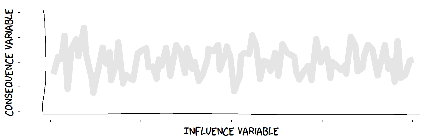
(With some definitions of “chaotic”, you can’t even draw a graph because, however close-up you look, there is no continuity at all. To the extent that an influence is completely chaotic, knowing about the influence adds no information at all.)
Combined influences: INUS causes
FundamentalsHere, we are not very interested in the debate about whether the INUS configuration is the right place to look for “the cause” of something. Partly because we are not so interested in deciding whether something is the cause or not – there are various cultural, legal and ethical issues involved which are not so important to evaluators. Most importantly because we have a more general and powerful way of “calculating” effects and impacts.

So-called “INUS” causes (“necessary part of a sufficient condition”) are interesting (???).
ℹ It is easy to realize them in Theorymaker - we use false/true Variables. The matches are part of an INUS condition and (therefore?) are supposed to count as a cause of the clothes drying, because they are a necessary part of a sufficient contribution, (i.e. part of a set of false/true Variables joined by “AND” leading to another set joined by “OR”). And it’s true that IF the electric heater is not also switched on (shown by the cross), and dry wood is indeed available (shown by the tick), THEN changes in the intervention Variable (striking the match) are matched by changes in the downstream consequence Variable (clothes are dried). But, from the broader perspective of causal networks this doesn’t seem to be specially remarkable: The underlying idea is, roughly: X counts as a cause of Y (given certain conditions) if when you manipulate X, this makes a corresponding difference in Y. This was in any case the motivation for saying the match was a cause of the clothes drying, and it’s all we really need. INUS configurations just make life more complicated. Causal networks do not “define” cause in this way; rather, causation is a primitive idea at the heart of each simple Theory. In causal networks, all we need to worry about is how to “calculate” causal influence further downstream in a causal network.
- it fails in a different context, e.g. when the heater is in fact on
- it only applies to causal networks consisting only of false/true Variables, which is rather restrictive
- there are other Variables in these or other configurations which could equally claim to be “a cause” but are not “INUS”, for example, in this configuration, the electric fire.
Hierarchical Logic Models

It is easy to make a hierarchical logic model in Theorymaker - one which divides a project into neat layers or slices (“outputs”, “outcomes” etc). This is a real-life example is from the IFRC. Note the boxes are not shown in the original but they do help to make things clearer.
Fuzzy Cognitive Maps

Fuzzy Cognitive Maps are fully realizable in Theorymaker.
This is a classic example: Rod Taber’s FCM on the American drug market (Taber 1991). Each of these Variables is conceived of as stretching over time, so could be preceded with a “~” symbol in Theorymaker.
It is not quite clear in this example to what extent the state of these Variables at any one moment depends only on the incoming arrows or also on their own state in a previous instant(s). If the latter, they should be marked with the “<U+21BA>” symbol in Theorymaker.
The key property of FCMs is that they use fuzzy logic to express and calculate the levels of the Variables. In the original version of this FCM, each Variable had just three levels: -1,0, or +1. Some FCMs use {-1,-0.5,0,+0.5,+1}.
Stock-and-Flow Diagrams
At first glance, systems diagrams are not amenable to being translated into functional networks because the arrows do not represent causal relations but are like pipes for transferring material. But we saw earlier that a flow can be translated into a pair of more basic Theorymaker concepts: an “Upstream” influence on the upstream Variable and a “Downstream” influence on the downstream Variable, see earlier.
Example: Teacher training

Example: Innovation projects

No need to divide a Theory into “Outputs & Outcomes”

In real life, Variables do not fit neatly into slices. Claiming otherwise is just “fake science”.

… the laptops also directly contribute to improved exam results, perhaps because the students can revise better: add an arrow - it is shown black here.
Students receive laptops is both one step and two steps away from the final outcome. So the “slices” structure breaks down.
No need to divide a Theory into “phases”

Here, the activities in each slice are supposed to take a specific amount of time and each completes before the next starts: the slices are phases.
Sometimes useful, sometimes a painful straightjacket.
The Prime Minister calls snap elections in two weeks, my party has to launch a campaign to influence a whole nation’s behaviour in 14 days:

Continuous Variables can stretch over time, and discrete Variables can repeat, and their timings can overlap one another in different ways.
Position tells you nothing about duration

A Theory is forced into slices. We are supposed to understand that the Variables in the later slices such as the final Outcome(s) are necessarily “longer-term” and will last or sustain longer.
Sometimes useful, sometimes a painful straightjacket.
Making a difference can take minutes or centuries, and the Difference can then last for minutes or centuries. Depends on many things but not a Variable’s position in a Theory.
Sustainable social change is hard but not because it is so many links away in some Theory.
Breaking up orthodox Theories of Change
In Logical Frameworks, Variables are divided up into slices: Inputs, Outputs, Outcomes etc. This is a very powerful simplification:
- The first slice is just the Variables we can control (called “Activities”, etc)
- The final slice is just the Variable(s) we really value (called “Goal”, etc)
- The slices “happen” one after another …

Theorymaker suggests some symbols to help you still identify the Variables we control and the Variables we value, as well as giving an indication of when things happen, without having to stick to such a rigid format.
- Valued Variables: ♥ (Or a 🙁 for things you don’t want)
- Variables you can control: ►
- Sketch out the timings with
^,~and_.
Be careful with Variables defined in terms of others
As soon as you start to combine different ideas about a project or a set of overlapping projects (for example when combining Theories from multiple stakeholders), you will find that some Variables overlap each other or have complicated relationships with one another - not just causal relationships but definitional. Ideally, we would reduce them all to a single set of independently measurable Variables and possibly another set of Variables which are defined in terms of the first set. But this can be really challenging.

To take a very simple example, how is “Improving overall happiness” related to “Countering self-harm”? Happiness surely has causal influences on probability of self-harm, and self-harm not only in an individual but also in the family will certainly lower happiness …
But absence of self-harm could also be part of the definition of happiness. It will probably be very difficult to include both these Variables in the same diagram.
Either all or none of your Variables should mention targets or changes or Differences
Indicators should never mention targets (DFID 2011). But often it is very useful if our Variables also include targets. A target should in general be thought of as a Difference; it can make sense to express a target in terms only of the Factual level if and only if the baseline is unlikely to change without the intervention. Otherwise you need to consider the Counterfactual too.

The problem is that the two intermediate Variables are just shown with Variable names whereas the others are also expressed in terms of Differences.
If you take this at face value, this will give you endless headaches down the line.
Two solutions:


Don’t say lower when you mean opposite of

Obviously we want to maximise the first two Variables in this chain, and minimise the last - it points in the opposite direction. So we use a word like ‘lower’ to make the switch of direction clear. But the first two rectangles just show the names of the Variables, whereas the third now includes a word ‘lower’ which seems also to talk about the difference made by the programme. Bad practice.
There is no obvious word which means the opposite of ‘mortality’. ℹ We can say ‘surviving’ but that isn’t an exact opposite - how do you count the number of children surviving? When?
Either all of your Variables should mention changes or Differences, or none of them should.
So use the “⊖” symbol, or the words ‘opposite of’.

… or show that this is an “minus” influence: ℹSo rather than a plus influence on an inverted Variable, the next example is an minus or “opposite direction” influence on a normal Variable.

… or mention the Differences made by the intervention on every Variable:

Don’t say “negative” when you mean “minus” (and don’t say “positive” when you mean “plus”)
We often hear about “negative” and “positive” influences in Theories – for example when talking about “positive” or “negative” feedback.
But as we can see from the example, this usage can be confusing when a Variable has a negative connotation. If you hear “bacteria have a positive influence on mortality” without knowing anything about the topic, you can’t be sure if the presence of bacteria means more people die, or fewer people? And if you hear that the medicine has “negative” influence mean that the medicine has subjectively negative consequences, i.e. more mortality?

In Theorymaker, we speak instead of “plus” and “minus” influences, and use the “⊕” and “⊖” symbols instead ℹ - The symbols usually go on the arrow, but they can go directly on the consequence Variable if there is only one influence Variable. . Now it is clear what we mean - more medicine means less mortality (minus), and more bacteria means more mortality (plus).

In Theorymaker, we use exactly the same terminology even in the case of false/true Variables. Below, there is a false/true influence Variable and even a false/true consequence Variable, but we can still think of this as an “minus” or “opposite” influence: if the patient is vaccinated, they don’t die.

Be careful with Variables which partially define others
A project’s activities lead to an increase in children’s musical creativity; the management want to show how that is a benefit for the donor’s broader focus, which is children’s creativity in general (defined as the average of creativity in several different domains, one of which is music):

General creativity is (partially) defined in terms of musical creativity, so a dashed arrow should be shown along with other factor(s) too, in order to complete the definition …
But at the same time, the project claims that more musical creativity also causes an increase in general creativity, which would seem to result in a link which is both causal and definitional at the same time: not a good idea. Instead, we can show a link from musical creativity to the other part(s) of the definition, like this:

Avoid passive sentences in Theories of Change

This is better:

We’d first go to the activists to gather data on the Variable.
But perhaps we don’t know who is going to do the monitoring, and that’s why we want to use the passive. We could say: “Somebody is monitoring city mayors”. But that is a “hard-to-search” Variable. Where would we go, what would we do, to gather data on that?
Don’t use a Variable to show a causal link

Breaks at least two rules:
- The arrows imply that A and B influence C; in fact A influences B and C just summarises that fact.
- The Variables in a Theory of Change should be free of causal words like “through” or “via” or “because”.

The causal story stands for itself.
We also used a grouping box to label the causal story (optional).
Don’t use a Variable to group project parts

This Theory fragment tries to use “Activities for teachers” and “Activities for students” as a way to organise the diagram. But this is wrong, because all arrows in a Theory of Change should show causal influence, and here the red arrows do not.
Just just eliminate the original Variables and use two grouping boxes instead:

One Variable can influence more than one other Variable

In lots of Theories of Change, especially those based on Logical Frameworks, every Variable only has one child Variable which it influences.
The “one child rule”
- is convenient for administrators
- allows us to number the Variables in our project hierarchically
- a convenient straight-jacket
But in real life … Of course a Variable can influence more than one other Variable!

Just because you’ve drawn a nice network diagram doesn’t mean you are dealing with a complex system …
Would you have guessed that the modern-looking network on the left has exactly the same structure as the boring, old-fashioned hierarchy on the right? ℹ The diagrams in these slides are nearly all produced by the dot layout engine in Graphviz. The dot engine tends not to produce circular layouts, but will find a hierarchy if there is one. That’s actually quite a useful thing to do when we’re thinking about cause and effect.

“Complex” and “System” are very buzzy buzz-words at the moment. We should check we don’t throw them around too much without thinking.

This structure does not show any features which might make us want to call it “complex”. In particular it doesn’t have any loops with negative feedback. Nor do we know enough about it yet to call it a “system” at all, or distinguish it from just any old bunch of Variables.
Simple recipes produce only predictable results?
Following a simple “recipe” is often given as a paradigm of a “simple system”, because doing so can’t lead to unpredictable results. But this is another complexity myth.

The eight pictures above are a really simple recipe for producing a pattern of black-and-white squares. You start with a big page of white squares, with a random pattern of black squares just in the top row. Then you colour each square in the second row according to these eight pictorial rules. So for example the first picture tells you if all three squares above are black, leave the square white. The next tells you that if just the square above and the square above and to the left are black, colour it black, and so on. Do this for all the squares, then repeat for the third row, and so on, gradually filling your page. Such a simple recipe can surely only produce a simple pattern?
But an example of what emerges is on the right. A pattern “big white triangle of differing size” has emerged from nowhere. How big will the biggest one be? Will they disappear further down? Stephen Wolfram (2002) has spent much of his life studying such “simple” recipes.

For many such recipes, it is impossible to predict the behaviour in advance. This was proven mathematically early in the last century.
The simplest of recipes, when repeated across time and/or space, can produce unpredictable, even emergent behaviour.
The world is much more complex than it used to be?
Irene Ng speaks for many who write about “complex systems” when she says: “What has happened in the last 50 years is that we’ve been trying to use deterministic tools to achieve emergent outcomes, essentially because those are the only tools we have learnt (systems thinkers are still a minority unfortunately). We treat complex systems like complicated systems. We try to design, specify, impose, dictate when we should be designing, enabling, intervening, stablising.”
Is there any historical truth in this at all? Did, say, a midwife 50 years ago only know how to impose and dictate rather than intervene and stablise? Was, say, managing the Mongol Empire, or Alexander’s conquests, a merely complicated, not complex task?

An often-used example of a complex task is bringing up a child (and I’d agree, loosely). Well, did we have no children to bring up until our frightfully modern era?
Perhaps Irene Ng is writing about our writing about management, not how it is or was actually done. But there are ancient books like “The Art of War” about how to lead, and manage, and reach goals. Were they all merely guides to snapping together simple solutions? Of course not.
Adaptive management is the new panacea?
Adaptive management won’t help you much if you have local minima or maxima.

Suppose you are at the point labelled “current” and don’t have an actual map of the area. All you can do is sense which direction takes you most steeply upwards. Then you can follow the adaptive management rule “always follow the path which leads upwards”. You’ll end up at a local high-point but you’ll miss the actual highest point.
And it won’t help you much if the outcome you value is later in time and the Variables you can monitor continuously aren’t strong predictors of it.